Stock Market Volatility

Key Learning:

• Broad and granular simulation
• Extracting and graphing results

The Problem

How likely is it for a medium-low volatile stock to crash in the market each year?

Specifications:

• +/-1.5% market price per day
• Initial stock price of $100

Solving the Problem

Simulation Core

A single sprout will represent a single year. The core simulation (plant) will random step each day for 365 days changing their current price by +/- the volatility. After a 'years' worth of simulating daily price changes, we will save the lowest reached price over the year as a bud equivalent to the percentage drop from initial price.

To save stock parameters into the class, we use a setup method instead of calling on __init__ since the Planter class is a sub-class of the Rust class PlanterLab, and will throw errors if you add any parameters to the __init__ method.

from seedler import *
import pandas as pd
import plotly.express as px

MAX_DRAWDOWN = 0

class MarketPlanter(Planter):
    def setup(self, initial_price, volatility, days):
        self.start = initial_price
        self.vol = volatility
        self.days = days
        return self

    def plant(self, sprout: Sprout):
        current_price = self.start
        lowest_price = self.start

        for _ in range(self.days):
            move = sprout.growth(-100, 100) / 100.0 
            current_price *= (1 + (move * self.vol))

            if current_price < lowest_price:
                lowest_price = current_price

        drawdown = ((self.start - lowest_price) / self.start) * 100
        sprout.add_bud(MAX_DRAWDOWN, int(drawdown))

    def plant_verbose(self, sprout: Sprout):
        current_price = self.start

        for day in range(self.days):
            move = sprout.growth(-100, 100) / 100.0 
            current_price *= (1 + (move * self.vol))

            change = (current_price / self.start) * 100
            sprout.add_bud(day, int(change))

The plant_verbose method is nearly identical to the plant method, and will be used for single-seed simulation later to retreive each day's price.

Filtering

To improve performance, we will only save seeds that drop below a specific price-drop threshhold. For this simulation, we will treat a 40% drop as a crash in the market.

class FindBlackSwan(Fire):
    def __init__(self, threshold=40):
        self.threshold = threshold

    def purge(self, sprout: Sprout):
        return sprout.get_bud_count(MAX_DRAWDOWN) < self.threshold

Running the Simulation

Each crash is recorded after the simulation, we can find the chance of crashing each year by dividing total recorded crashes by the number of simulations run.

sims = 50_000

lab = MarketPlanter().setup(initial_price=100, volatility=0.015, days=356)
crashes = lab.find_seeds(fire=FindBlackSwan(40), maximum=sims)

crash_chance = len(crashes) / sims * 100

print(f"Crashes (down 40%, vol {lab.vol}): {crash_chance:>6.2f}% ({len(crashes)}/{sims})")

Output

Crashes (down 40%, vol 0.15):   0.21% (106/50000)

Given our current simulation, the market is extremely unlikely to crash in a single given year.

Plotting Crashes

Taking this further, we can plot the daily price over the course of a year for each crash that occurred. This can be helpful to get a sense of how the market reaches a point where it crashes.

We start by re-simulating all crashing seeds, and collecting the per-day price, using the plant_verbose method.

if len(crashes) == 0: quit

# Limiting total crashes plotted for graph performance
target_seeds = [c[0] for c in crashes[:200]]

all_paths = []

for seed_id in target_seeds:
    sprout = Sprout(seed_id)
    lab.plant_verbose(sprout)

    temp_df = pd.DataFrame(sprout.to_dict().items(), columns=['day', 'perc'])
    temp_df['seed'] = str(seed_id)  # Add seed ID as a label for Plotly
    all_paths.append(temp_df)

df_master = pd.concat(all_paths).sort_values(by=['seed', 'day']).reset_index(drop=True)

Then we graph the results.

GraphPython

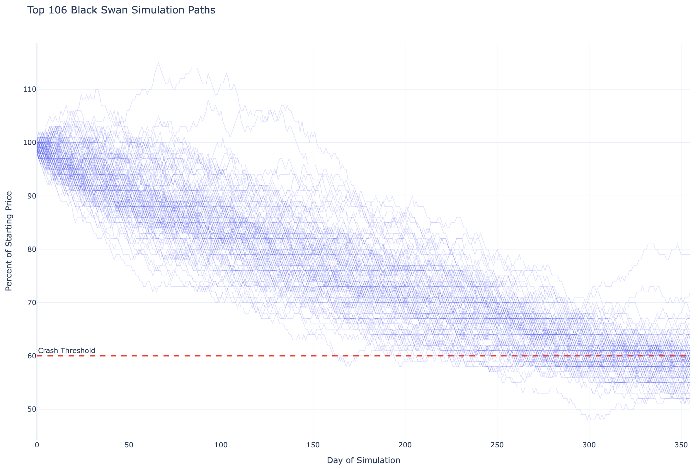
fig = px.line(
    df_master, 
    x="day", 
    y="perc", 
    line_group="seed",
    title=f"Top {len(target_seeds)} Black Swan Simulation Paths",
    template="plotly_white",
    render_mode="webgl"
)

fig.update_traces(
    line=dict(color="rgba(100, 110, 250, 0.2)", width=1),
    hoverlabel=dict(bgcolor="white"),
    hovertemplate="Seed: %{customdata[0]}<br>Day: %{x}<br>Percent: %{y}%<extra></extra>",
    customdata=df_master[['seed']]
)

fig.add_hline(
    y=60.0, 
    line_dash="dash", 
    line_color="red", 
    annotation_text="Crash Threshold",
    annotation_position="top left"
)

fig.update_layout(
    hovermode="closest",
    showlegend=False,
    yaxis_title="Percent of Starting Price",
    xaxis_title="Day of Simulation"
)

fig.show()

As we can see from the graph, Every crash is a slow-burn throughout the year, only crashing towards the end of the year.

Answering the Problem

According to our simulation with the given parameters, a 1.5% daily volatile stock has a ~0.21% chance of crashing in a given year.